Which layout of an advertisement leads to more clicks? Would a different color or position of the purchase button lead to a higher conversion rate? Does a special offer really attract more customers – and which of two phrasings would be better? For a long time, people have trusted their gut feeling to answer these questions. Today all these questions could be answered by conducting an A/B test. For this purpose, visitors of a website are randomly assigned to one of two groups between which the target metric (i.e. click-through rate, conversion rate…) can then be compared. Due to this randomization, the groups do not systematically differ in all other relevant dimensions. This means: If your target metric takes a significantly higher value in one group, you can be quite sure that it is because of your treatment and not because of any other variable. In comparison to other methods, conducting an A/B test does not require extensive statistical knowledge. Nevertheless, some caveats have to be taken into account. When making a statistical decision, there are two possible errors (see also table 1): A Type I error means that we observe a significant result although there is no real difference between our groups. A Type II error means that we do not observe a significant result although there is in fact a difference. The Type I error can be controlled and set to a fixed number in advance, e.g., at 5%, often denoted as α or the significance level. The Type II error in contrast cannot be controlled directly. It decreases with the sample size and the magnitude of the actual effect. When, for example, one of the designs performs way better than the other one, it’s more likely that the difference is actually detected by the test in comparison to a situation where there is only a small difference with respect to the target metric. Therefore, the required sample size can be computed in advance, given α and the minimum effect size you want to be able to detect (statistical power analysis). Knowing the average traffic on the website you can get a rough idea of the time you have to wait for the test to complete. Setting the rule for the end of the test in advance is often called “fixed-horizon testing”. Table 1: Overview over possible errors and correct decisions in statistical tests Effect really exists No Yes Statistical test is significant No True negative Type II error (false negative) Yes Type I error (false positive) True positive Statistical tests generally provide the p-value which reflects the probability of obtaining the observed result (or an even more extreme one) just by chance, given that there is no effect. If the p-value is smaller than α, the result is denoted as “significant”. When running an A/B test you may not always want to wait until the end but take a look from time to time to see how the test performs. What if you suddenly observe that your p-value has already fallen below your significance level – doesn’t that mean that the winner has already been identified and you could stop the test? Although this conclusion is very appealing, it can also be very wrong. The p-value fluctuates strongly during the experiment and even if the p-value at the end of the fixed-horizon is substantially larger than α, it can go below α at some point during the experiment. This is the reason why looking at your p-value several times is a little bit like cheating, because it makes your actual probability of a Type I error substantially larger than the α you chose in advance. This is called “α inflation”. At best you only change the color or position of a button although it does not have any impact. At worst, your company provides a special offer which causes costs but actually no gain. The more often you check your p-value during the data collection, the more likely you are to draw wrong conclusions. In short: As attractive as it may seem, don’t stop your A/B test early just because you are observing a significant result. In fact you can prove that if you increase your time horizon to infinity, you are guaranteed to get a significant p-value at some point in time. The following code simulates some data and plots the course of the p-value during the test. (For the first samples which are still very small R returns a warning that the chi square approximation may be incorrect.) library(timeDate) library(ggplot2) # Choose parameters: pA