linear-algebra
Matrix Product Interpretations and Visualizations: Learn Linear Algebra from scratch. Build a foundation for Machine Learning and other key technologies.
MatrixCalculus provides matrix calculus for everyone. It is an online tool that computes vector and matrix derivatives (matrix calculus).
Part 4: A comprehensive step-by-step guide to solving a linear system with LU Decomposition

An eigenvalue of a square matrix $LATEX A$ is a scalar $latex \lambda$ such that $latex Ax = \lambda x$ for some nonzero vector $latex x$. The vector $latex x$ is an eigenvector of $LATEX A$ and it…
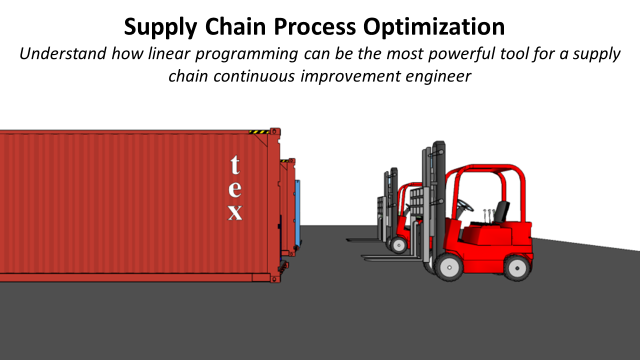
Understand how linear programming can be the most powerful tool for a supply chain continuous improvement engineer
In this article, we discuss the importance of linear algebra in data science and machine learning.
Quantifying Uncertainty in Computation.

This article gives an introduction to vector norms, vector distances and their application in the field of data science

In January 2016, I was honored to receive an “Honorable Mention” of the John Chambers Award 2016. This article was written for R-bloggers, whose builder, Tal Galili, kindly invited me to write an introduction to the rARPACK package. A Short Story of rARPACK Eigenvalue decomposition is a commonly used technique in numerous statistical problems. For example, principal component analysis (PCA) basically conducts eigenvalue decomposition on the sample covariance of a data matrix: the eigenvalues are the component variances, and eigenvectors are the variable loadings. In R, the standard way to compute eigenvalues is the eigen() function. However, when the matrix becomes large, eigen() can be very time-consuming: the complexity to calculate all eigenvalues of a $n times n$ matrix is $O(n^3)$. While in real applications, we usually only need to compute a few eigenvalues or eigenvectors, for example to visualize high dimensional data using PCA, we may only use the first two or three components to draw a scatterplot. Unfortunately in eigen(), there is no option to limit the number of eigenvalues to be computed. This means that we always need to do the full eigen decomposition, which can cause a huge waste in computation. And this is why the rARPACK package was developed. As the name indicates, rARPACK was originally an R wrapper of the ARPACK library, a FORTRAN package that is used to calculate a few eigenvalues of a square matrix. However ARPACK has stopped development for a long time, and it has some compatibility issues with the current version of LAPACK. Therefore to maintain rARPACK in a good state, I wrote a new backend for rARPACK, and that is the C++ library Spectra. The name of rARPACK was POORLY designed, I admit. Starting from version 0.8-0, rARPACK no longer relies on ARPACK, but due to CRAN polices and reverse dependence, I have to keep using the old name. Features and Usage The usage of rARPACK is simple. If you want to calculate some eigenvalues of a square matrix A, just call the function eigs() and tells it how many eigenvalues you want (argument k), and which eigenvalues to calculate (argument which). By default, which = "LM" means to pick the eigenvalues with the largest magnitude (modulus for complex numbers and absolute value for real numbers). If the matrix is known to be symmetric, calling eigs_sym() is preferred since it guarantees that the eigenvalues are real. library(rARPACK) set.seed(123) ## Some random data x = matrix(rnorm(1000 * 100), 1000) ## If retvec == FALSE, we don't calculate eigenvectors eigs_sym(cov(x), k = 5, which = "LM", opts = list(retvec = FALSE)) For really large data, the matrix is usually in sparse form. rARPACK supports several sparse matrix types defined in the Matrix package, and you can even pass an implicit matrix defined by a function to eigs(). See ?rARPACK::eigs for details. library(Matrix) spmat = as(cov(x), "dgCMatrix") eigs_sym(spmat, 2) ## Implicitly define the matrix by a function that calculates A %*% x ## Below represents a diagonal matrix diag(c(1:10)) fmat = function(x, args) { return(x * (1:10)) } eigs_sym(fmat, 3, n = 10, args = NULL) From Eigenvalue to SVD An extension to eigenvalue decomposition is the singular value decomposition (SVD), which works for general rectangular matrices. Still take PCA as an example. To calculate variable loadings, we can perform an SVD on the centered data matrix, and the loadings will be contained in the right singular vectors. This method avoids computing the covariance matrix, and is generally more stable and accurate than using cov() and eigen(). Similar to eigs(), rARPACK provides the function svds() to conduct partial SVD, meaning that only part of the singular pairs (values and vectors) are to be computed. Below shows an example that computes the first three PCs of a 2000x500 matrix, and I compare the timings of three different algorithms: library(microbenchmark) set.seed(123) ## Some random data x = matrix(rnorm(2000 * 500), 2000) pc = function(x, k) { ## First center data xc = scale(x, center = TRUE, scale = FALSE) ## Partial SVD decomp = svds(xc, k, nu = 0, nv = k) return(list(loadings = decomp$v, scores = xc %*% decomp$v)) } microbenchmark(princomp(x), prcomp(x), pc(x, 3), times = 5) The princomp() and prcomp() functions are the standard approaches in R to do PCA, which will call eigen() and svd() respectively. On my machine (Fedora Linux 23, R 3.2.3 with optimized single-threaded OpenBLAS), the timing results are as follows: Unit: milliseconds expr min lq mean median uq max neval princomp(x) 274.7621 276.1187 304.3067 288.7990 289.5324 392.3211 5 prcomp(x) 306.4675 391.9723 408.9141 396.8029 397.3183 552.0093 5 pc(x, 3) 162.2127 163.0465 188.3369 163.3839 186.1554 266.8859 5 Applications SVD has some interesting applications, and one of them is image compression. The basic idea is to perform a partial SVD on the image matrix, and then recover it using the calculated singular values and singular vectors. Below shows an image of size 622x1000: (Orignal image) If we use the first five singular pairs to recover the image, then we need to store 8115 elements, which is only 1.3% of the original data size. The recovered image will look like below: (5 singular pairs) Even if the recovered image is quite blurred, it already reveals the main structure of the original image. And if we increase the number of singular pairs to 50, then the difference is almost imperceptible, as is shown below. (50 singular pairs) There is also a nice Shiny App developed by Nan Xiao, Yihui Xie and Tong He that allows users to upload an image and visualize the effect of compression using this algorithm. The code is available on GitHub. Performance Finally, I would like to use some benchmark results to show the performance of rARPACK. As far as I know, there are very few packages available in R that can do the partial eigenvalue decomposition, so the results here are based on partial SVD. The first plot compares different SVD functions on a 1000x500 matrix, with dense format on the left panel, and sparse format on the right. The second plot shows the results on a 5000x2500 matrix. The functions used corresponding to the axis labels are as follows: svd: svd() from base R, which computes the full SVD irlba: irlba() from irlba package, partial SVD propack, trlan: propack.svd() and trlan.svd() from svd package, partial SVD svds: svds() from rARPACK The code for benchmark and the environment to run the code can be found here.
Multiplying matrices is among the most fundamental and compute-intensive operations in machine learning. Consequently, there has been significant work on efficiently approximating matrix...

Poisson's Equation is an incredibly powerful tool...
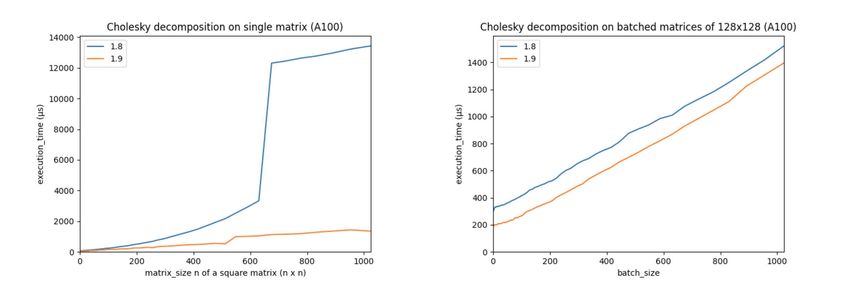
Linear algebra is essential to deep learning and scientific computing, and it’s always been a core part of PyTorch. PyTorch 1.9 extends PyTorch’s support for linear algebra operations with the torch.linalg module. This module, documented here, has 26 operators, including faster and easier to use versions of older PyTorch operators, every function from NumPy’s linear algebra module extended with accelerator and autograd support, and a few operators that are completely new. This makes the torch.linalg immediately familiar to NumPy users and an exciting update to PyTorch’s linear algebra support.

Current custom AI hardware devices are built around super-efficient, high performance matrix multiplication. This category of accelerators includes the
Free online textbook of Jupyter notebooks for fast.ai Computational Linear Algebra course - fastai/numerical-linear-algebra
Linear algebra is foundational in data science and machine learning. Beginners starting out along their learning journey in data science--as well as established practitioners--must develop a strong familiarity with the essential concepts in linear algebra.
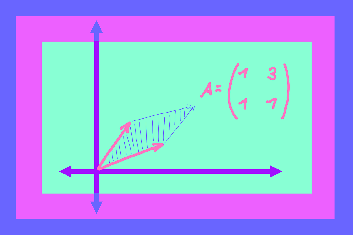
The geometric intuition behind determinants could change how you think about them.
Intuitive Math Descriptions
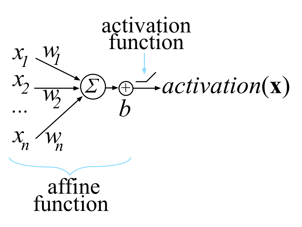
Most of us last saw calculus in school, but derivatives are a critical part of machine learning, particularly deep neural networks, which are trained by optimizing a loss function. This article is an attempt to explain all the matrix calculus you need in order to understand the training of deep neural networks. We assume no math knowledge beyond what you learned in calculus 1, and provide links to help you refresh the necessary math where needed.

All of the Linear Algebra Operations that You Need to Use in NumPy for Machine Learning. The Python numerical computation library called NumPy provides many linear algebra functions that may be useful as a machine learning practitioner. In this tutorial, you will discover the key functions for working with vectors and matrices that you may find useful as a machine…