Perfectly Awesome

So, if you’ve ever asked, “How long until X happens?” and wanted to back that up with solid data, you’re in the right place.

The Kaplan-Meier survival curve estimator is one of the most cited ideas in science

Survival analysis consists of statistical methods that help us understand and predict how long it takes for an event to occur.

Pic by author - using DALL-E 3 When running experiments don’t forget to bring your survival kit I’ve already made the case in several blog posts (part 1, part 2, part 3) that using survival analysis can improve churn prediction. In this blog post I’ll ...

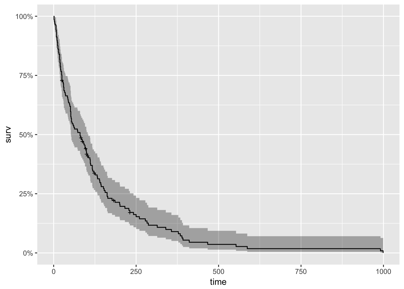
With roots dating back to at least 1662 when John Graunt, a London merchant, published an extensive set of inferences based on mortality records, survival analysis is one of the oldest subfields of Statistics [1]. Basic life-table methods, including techniques for dealing with censored data, were discovered before 1700 [2], and in the early eighteenth century, the old masters - de Moivre working on annuities, and Daniel Bernoulli studying competing risks for the analysis of smallpox inoculation - developed the modern foundations of the field [2]. Today, survival analysis models are important in Engineering, Insurance, Marketing, Medicine, and many more application areas. So, it is not surprising that R should be rich in survival analysis functions. CRAN’s Survival Analysis Task View, a curated list of the best relevant R survival analysis packages and functions, is indeed formidable. We all owe a great deal of gratitude to Arthur Allignol and Aurielien Latouche, the task view maintainers. Looking at the Task View on a small screen, however, is a bit like standing too close to a brick wall - left-right, up-down, bricks all around. It is a fantastic edifice that gives some idea of the significant contributions R developers have made both to the theory and practice of Survival Analysis. As well-organized as it is, however, I imagine that even survival analysis experts need some time to find their way around this task view. Newcomers - people either new to R or new to survival analysis or both - must find it overwhelming. So, it is with newcomers in mind that I offer the following narrow trajectory through the task view that relies on just a few packages: survival, ggplot2, ggfortify, and ranger The survival package is the cornerstone of the entire R survival analysis edifice. Not only is the package itself rich in features, but the object created by the Surv() function, which contains failure time and censoring information, is the basic survival analysis data structure in R. Dr. Terry Therneau, the package author, began working on the survival package in 1986. The first public release, in late 1989, used the Statlib service hosted by Carnegie Mellon University. Thereafter, the package was incorporated directly into Splus, and subsequently into R. ggfortify enables producing handsome, one-line survival plots with ggplot2::autoplot. ranger might be the surprise in my very short list of survival packages. The ranger() function is well-known for being a fast implementation of the Random Forests algorithm for building ensembles of classification and regression trees. But ranger() also works with survival data. Benchmarks indicate that ranger() is suitable for building time-to-event models with the large, high-dimensional data sets important to internet marketing applications. Since ranger() uses standard Surv() survival objects, it’s an ideal tool for getting acquainted with survival analysis in this machine-learning age. Load the data This first block of code loads the required packages, along with the veteran dataset from the survival package that contains data from a two-treatment, randomized trial for lung cancer. library(survival) library(ranger) library(ggplot2) library(dplyr) library(ggfortify) #------------ data(veteran) head(veteran) ## trt celltype time status karno diagtime age prior ## 1 1 squamous 72 1 60 7 69 0 ## 2 1 squamous 411 1 70 5 64 10 ## 3 1 squamous 228 1 60 3 38 0 ## 4 1 squamous 126 1 60 9 63 10 ## 5 1 squamous 118 1 70 11 65 10 ## 6 1 squamous 10 1 20 5 49 0 The variables in veteran are: * trt: 1=standard 2=test * celltype: 1=squamous, 2=small cell, 3=adeno, 4=large * time: survival time in days * status: censoring status * karno: Karnofsky performance score (100=good) * diagtime: months from diagnosis to randomization * age: in years * prior: prior therapy 0=no, 10=yes Kaplan Meier Analysis The first thing to do is to use Surv() to build the standard survival object. The variable time records survival time; status indicates whether the patient’s death was observed (status = 1) or that survival time was censored (status = 0). Note that a “+” after the time in the print out of km indicates censoring. # Kaplan Meier Survival Curve km

Understand survival analysis, its use in the industry, and how to apply it in Python

Learn more about survival analysis (also called time-to-event analysis) and how it is used, and how to apply it by hand and in R

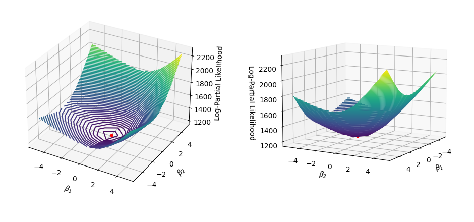
Finding the coefficients that maximize the log-partial likelihood in Python

Making a survival analysis can be a challenge even for experienced R users, but the good news is I’ll help you make beautiful, publication-quality survival plots in under 10-minutes. Here’s what WE are going to do: Make your first survival model an...

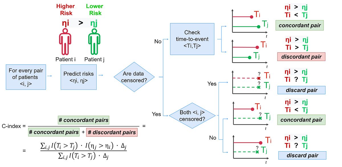
Introduction to the most popular performance evaluation metrics for survival analysis along with practical Python examples

An initial look into the method best suited for examining time-to-event data

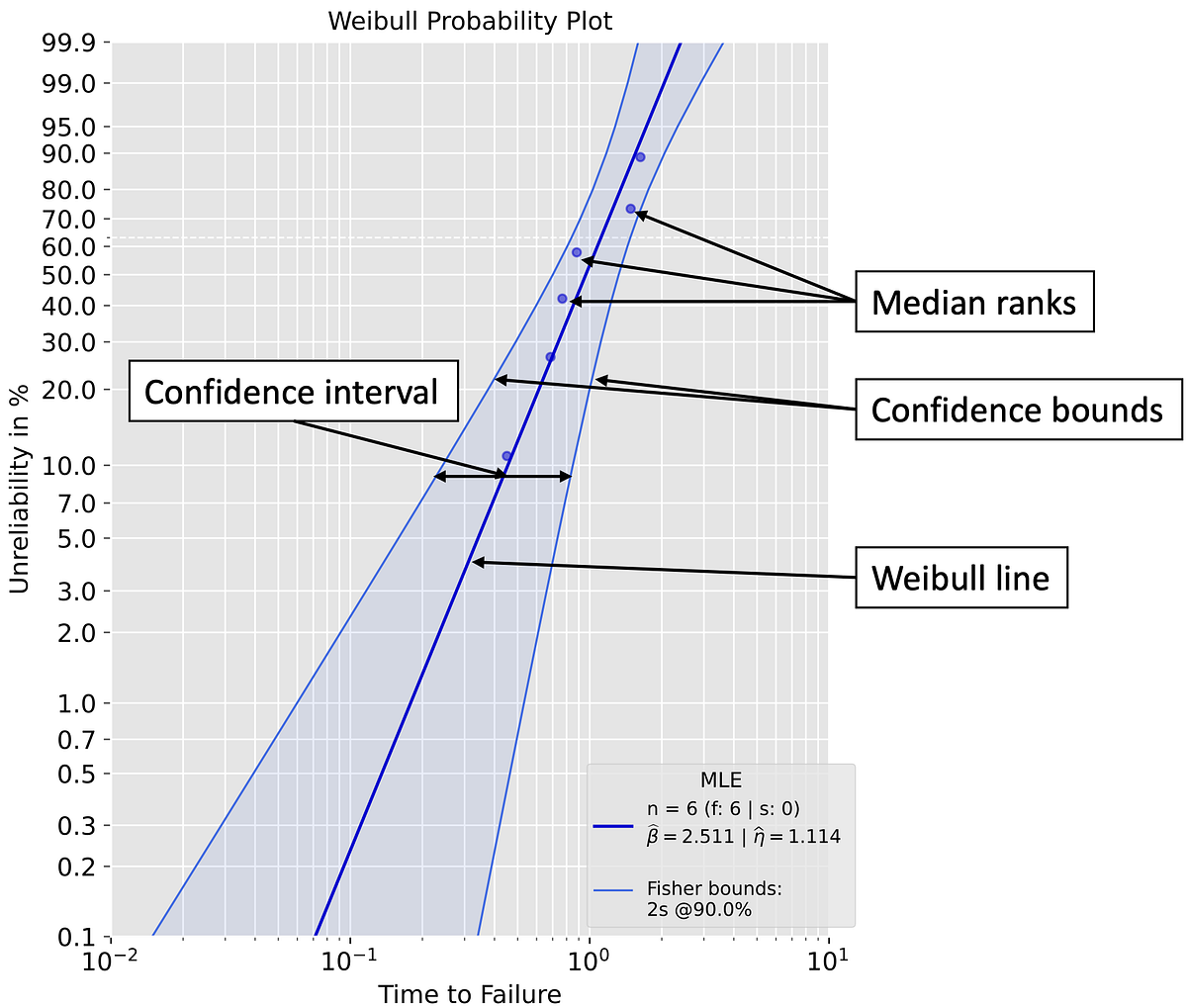
A Quick Guide to The Weibull Analysis

In Cows using R

What companies can learn from employee turnover data

Concluding this three-part series covering a step-by-step review of statistical survival analysis, we look at a detailed example implementing the Kaplan-Meier fitter based on different groups, a Log-Rank test, and Cox Regression, all with examples and shared code.

Learn one of the most popular techniques used for survival analysis and how to implement it in Python!

With worked out examples using Python and Lifelines